Adam Gruber's Adventure in Data Science

by Adam Gruber

15.4 million new personal vehicles will be sold in the USA in 2023. Cars are one of the most significant purchases the average person makes several times in their life. Each purchase is a chance to gain or lose lifelong customers. High potential profits or huge losses if cars are not correctly valued on the market. Inventory costs are very high for a dealership. Dealerships, car websites, re-sellers, consumers, and more all have a vested interest in properly estimating prices. Industry journals like Kelly Blue Book are trusted for their guidance on pricing.

We are attempting to predict the retail price for cars. The data set has a very wide range of car prices. It ranges from $10,280 to a max price of $192,465. We decided to transform the data for elastic regression using the caret package. We used the function to scale and center the inputs.  The columns Sport, SUV, Wagon, and Minivan were converted to factor. Each of these categories is an indicator of certain traits. Height was converted to numeric.

The data set had many missing values. They were in MPG, Cylinders, Wheelbase, Weight, Length, and Height. The data set was very small with only 428 observations. Height was missing 28 values. If we omitted Height, we would omit 6.5% of the data from one column. Overall, only 90% of the observations had no missing values. This was not enough to remove incomplete predictors; we felt keeping them all would produce the best model. This can be seen in the graph which columns had missing data and which did not. This is also a list of all predictors used.

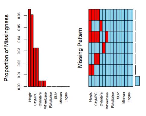
To keep as much data as possible, the missing values were imputed using the MICE package in R. This package assumed the missing values were related to the remaining columns. The other columns are used as predictors. This makes sense since the MPG was missing for a car with 500 HP. This car should have a lower MPG compared to the mean (20). The imputed value was 17. This is why we can not just merely apply mean/median across the missing data. This would heavily reduce the data points on the outskirts, reducing our predictive abilities.

Elastic regression was chosen for a few reasons. Elastic Net regression can select which predictors matter the most and which are noise. It can reduce the coefficient of unneeded terms to 0. This takes them out of the model. This is useful when there are many predictors, and we are uncertain which ones will provide the most value. The data was scaled using the scale, center function in caret.  This allows a more interpretable model when looking at the value of certain attributes.  The manufacturers and consumers want to know the value of increased cylinders has.

Robust Regression should be used when there are many outliers in the data set. Individual outliers can be weighted so they no longer affect the model as much. This is important for this data set when we have many different models of cars. We did not transform the data set for robust regression.  There are several outliers if we use only a non-transformed linear model to predict Retail Price. The Residuals vs Fitted model show a heavy concentration of residuals to the left side rather than evenly spread out. The Q-Q residual plot shows several outliers near the tail-ends of the plot. This is likely due to high-end sports cars and the more compact cars. Observations 428 and 424 were high-end sports cars. 

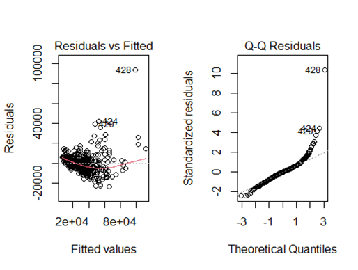
We must select the optimal lambda and alpha when performing elastic net regression. I chose to fit over 100 alpha and 100 lambdas. The optimal alpha was .01 and lambda was 7.389. This was found using 10-fold cross-validation with the Caret package. To prepare the data for elastic net regression, the data needed to be scaled and centered. This reduces the right skewness as seen in the Residuals vs Fitted Plot. The RSME was 9646. This is a very high error rate. But when considering how varied the data set is, it makes sense.

The robust regression does not need the data to be transformed since each data point is weighted differently. Using ten-fold cross-validation, the RSME is 9802. This is significantly worse than the Elastic Net Regression model. We can compare them using double cross-validation to see if Robust Regression can produce a better model.

Double Cross validation showed Elastic Net to be the best model again with an RSME of 9684. This is expected since the double cross-validation has increased sampling to reduce overfitting. This increases the error rate. But produces a more honest model when using testing data.

Method	Single_CV_RMSE	Double_CV_RMSE
Elastic	9,646	9,684
Robust	9,802	10,095

Our final model explained 84% of the variation for Retail Price. This seems to be a reasonable model when considering how varied our data set is. This means our model would suit most of the data but struggle with the outliers. Many of those appear to be specific models of cars that go against the rest of the data. There are ways to improve the model, which will be discussed later.

Model_Predictor	Coef_value
Intercept	32,880.89
Type Other	-1,323.22
Type RWD	1,996.30
Sport 1	226.83
SUV 1	-928.61
Wagon 1	-531.10
Minivan 1	514.98
Pickup 1	-1,485.63
Engine	-4,033.75
Cylinders	2,835.02
Horsepower	16,026.69
City MPG	-381.22
HWY MPG	3,541.58
Weight	7,436.30
Wheelbase	-5,173.99
Length	1,546.52
Height	-2,805.88

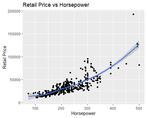
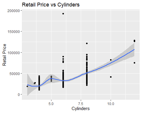
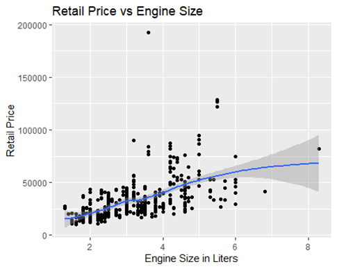
The three most important predictors are engine, cylinders, and horsepower. The most important is horsepower. They have positive coefficients. This makes sense when considering the highest-priced cars have higher HP, Cylinders, and Engine size. This positive correlation can be seen in the graphs. These scatter plots also show the many outliers influencing the smoothing curve. This shows the general trend and why we must account for the outliers. The most expensive are sports cars, and they are likely to have all high levels of all 3 of these. Another highly negative coefficient was height. This was surprising, but it makes sense when the top prices are sports cars. They tend to be lower heights and more aerodynamic.

The data set is small and the value we are trying to predict has a very wide range: $12,000 – $192,000. There are many kinds of cars in the model making predictions harder.

Comparing to  Other Models

Car price prediction is a problem that has been tackled in many different papers before. Enis Gegic et.al used a neural network to classify cars in their paper “Car Price Prediction using Machine Learning Techniques.” In this paper, they broke down the price into ranges. This allowed them to have low, medium, and high price categories. These were further broken down into 15 price categories. They used data from 2014 for cars sold in Bosnia and Herzegovina. They used the predictors such as brand, model, fuel, car condition, and features. The only predictors in common to our model are power and drive.

This classification technique allowed them to be more accurate, with 90.48% when working with only the expensive category of cars. They can achieve this high accuracy since they only classify expensive cars into five upper price ranges. Smaller price range categories are $1500 and the top ones are $20,000 range. They are not trying to predict the actual price of the cars. This gives their model limited uses since many experts can predict a Mercedes Benz S Class would be in the most expensive car category, but not the exact price it should be sold for. Their model struggled when trying to classify all the data at once. Instead, they divided it into low, medium, and high price categories. Then, they would predict just that segment.

Improving the Model

The model appears to explain 84% of the variation in the price accurately. This model seems satisfactory for generalizations but would need to be improved if we are going to use to for car dealerships. Our model could be enhanced by similarly only trying to predict the price of cars based on certain drive trains or price ranges. This would allow a more accurate prediction but require a more extensive data set to ensure a high level of accuracy.  The model could also benefit from including the Brand and model as well. Certain Brands are known for higher quality or certain prestige. People are willing to pay extra for those prestigious brands, which is not easily measured.

Specific unmeasured values are why the Retail Price is mostly correlated to the predictors but has a slightly causal relationship. Sometimes, a high price brings prestige.  Building a model that is more specific to certain types, brands, and attributes will build a more accurate model. A Toyota can have weight, cylinders, and horsepower similar to a Lexus. Both come from the same company. They will have wildly different prices. This is why the model needs a few more predictors to increase accuracy.

Several predictors should be added to the next study: location, Brand, and resale value. Location can make a difference for drive trains when comparing areas that value 4WD for snowy weather. The brand would help make it more accurate when predicting retail price since it can easily differentiate based on high or low-end brands. Resale value could also make a difference as well. Customers who know in several years, their car can be resold for a high value might be willing to spend more. This predictor was not seen in other papers.

The model could be redone with a Random Forest or neural network as Enis Gegic et al. did. This classification method seems accurate, but they created several categories of price ranges. The next step would be to reduce the price range to a $500 window. This could produce more errors, but it is a more helpful model for sellers and buyers to know the ideal price on the market.

Conclusion

Many people have been trying for years to accurately predict the price of cars, especially since they are one of the most significant purchases people make regularly. We built a model using all available predictors in our 04_cars data set. Using elastic net regression, and double cross validation, we could explain 84% of the variation in Retail Price for cars. Other researchers used neural networks to classify the cars into price ranges rather than specific dollar values. This seemed more accurate but could be less effective for specific parties like dealerships. They may need an exact model to price their vehicles effectively.